from bofire.data_models.features.api import (
    CategoricalDescriptorInput,
    CategoricalInput,
    ContinuousInput,
    DiscreteInput,
)


x1 = ContinuousInput(key="conc_A", bounds=[0, 1])
x2 = ContinuousInput(key="conc_B", bounds=[0, 1])
x3 = ContinuousInput(key="conc_C", bounds=[0, 1])
x4 = DiscreteInput(key="temperature", values=[20, 50, 90], unit="°C")

x5 = CategoricalInput(
    key="catalyst",
    categories=["cat_X", "cat_Y", "cat_Z"],
    allowed=[
        True,
        True,
        False,
    ],  # we have run out of catalyst Z, but still want to model past experiments
)

x6 = CategoricalDescriptorInput(
    key="solvent",
    categories=["water", "methanol", "ethanol"],
    descriptors=["viscosity (mPa s)", "density (kg/m3)"],
    values=[[1.0, 997], [0.59, 792], [1.2, 789]],
)Basic terminology
In the following it is showed how to setup optimization problems in BoFire and how to use strategies to solve them.
Setting up the optimization problem
In BoFire, an optimization problem is defined by defining a domain containing input and output features, as well as optionally including constraints.
Features
Input features can be continuous, discrete, categorical.
We also support a range of specialized inputs that make defining your experiments easier, such as: - CategoricalMolecularInput allows transformations of molecules to featurizations (Fingerprints, Fragments and more). - TaskInput enables transfer learning and multi-fidelity methods, where you have access to similar experiments that can inform your optimization. - *DescriptorInput gives additional information about its value, combining the data with its significance.
We can define both continuous and categorical outputs. Each output feature should have an objective, which determines if we aim to minimize, maximize, or drive the feature to a given value. Furthermore, we can define weights between 0 and 1 in case the objectives should not be weighted equally.
from bofire.data_models.features.api import ContinuousOutput
from bofire.data_models.objectives.api import MaximizeObjective, MinimizeObjective


objective1 = MaximizeObjective(
    w=1.0,
    bounds=[0.0, 1.0],
)
y1 = ContinuousOutput(key="yield", objective=objective1)

objective2 = MinimizeObjective(w=1.0)
y2 = ContinuousOutput(key="time_taken", objective=objective2)
In- and output features are collected in respective feature lists, which can be summarized with the get_reps_df method.
from bofire.data_models.domain.api import Inputs, Outputs


input_features = Inputs(features=[x1, x2, x3, x4, x5, x6])
output_features = Outputs(features=[y1, y2])

input_features.get_reps_df()| Type | Description | |
|---|---|---|
| conc_A | ContinuousInput | [0.0,1.0] |
| conc_B | ContinuousInput | [0.0,1.0] |
| conc_C | ContinuousInput | [0.0,1.0] |
| temperature | DiscreteInput | type='DiscreteInput' key='temperature' context... |
| solvent | CategoricalDescriptorInput | 3 categories |
| catalyst | CategoricalInput | 3 categories |
output_features.get_reps_df()| Type | Description | |
|---|---|---|
| time_taken | ContinuousOutput | ContinuousOutputFeature |
| yield | ContinuousOutput | ContinuousOutputFeature |
Individual features can be retrieved by name, and a collection of features can be retrieved with a list of names.
input_features.get_by_key("catalyst")CategoricalInput(type='CategoricalInput', key='catalyst', context=None, categories=['cat_X', 'cat_Y', 'cat_Z'], allowed=[True, True, False])input_features.get_by_keys(["catalyst", "conc_B"])Inputs(type='Inputs', features=[ContinuousInput(type='ContinuousInput', key='conc_B', context=None, unit=None, bounds=[0.0, 1.0], local_relative_bounds=None, stepsize=None, allow_zero=False), CategoricalInput(type='CategoricalInput', key='catalyst', context=None, categories=['cat_X', 'cat_Y', 'cat_Z'], allowed=[True, True, False])])Features of a specific type can be returned by the get method. By using the exact argument, we can force the method to only return features that match the class exactly.
input_features.get(CategoricalInput)Inputs(type='Inputs', features=[CategoricalDescriptorInput(type='CategoricalDescriptorInput', key='solvent', context=None, categories=['water', 'methanol', 'ethanol'], allowed=[True, True, True], descriptors=['viscosity (mPa s)', 'density (kg/m3)'], values=[[1.0, 997.0], [0.59, 792.0], [1.2, 789.0]]), CategoricalInput(type='CategoricalInput', key='catalyst', context=None, categories=['cat_X', 'cat_Y', 'cat_Z'], allowed=[True, True, False])])input_features.get(CategoricalInput, exact=True)Inputs(type='Inputs', features=[CategoricalInput(type='CategoricalInput', key='catalyst', context=None, categories=['cat_X', 'cat_Y', 'cat_Z'], allowed=[True, True, False])])The get_keys method follows the same logic as the get method, but returns just the keys of the features instead of the features itself.
input_features.get_keys(CategoricalInput)['solvent', 'catalyst']The input feature container further provides methods to return a feature container with only all fixed or all free features.
free_inputs = input_features.get_free()
fixed_inputs = input_features.get_fixed()
One can uniformly sample from individual input features.
x5.sample(2)0 cat_Y
1 cat_Y
Name: catalyst, dtype: strOr directly from input feature containers, uniform, sobol and LHS sampling is possible. A default, uniform sampling is used.
from bofire.data_models.enum import SamplingMethodEnum


X = input_features.sample(n=10, method=SamplingMethodEnum.LHS)

X| conc_A | conc_B | conc_C | temperature | solvent | catalyst | |
|---|---|---|---|---|---|---|
| 0 | 0.080308 | 0.347303 | 0.663096 | 20.0 | methanol | cat_Y |
| 1 | 0.688718 | 0.958925 | 0.362766 | 90.0 | water | cat_X |
| 2 | 0.525635 | 0.712967 | 0.082406 | 20.0 | ethanol | cat_X |
| 3 | 0.227042 | 0.661019 | 0.533140 | 90.0 | methanol | cat_Y |
| 4 | 0.133128 | 0.552323 | 0.168095 | 90.0 | water | cat_Y |
| 5 | 0.932419 | 0.864245 | 0.895975 | 50.0 | water | cat_X |
| 6 | 0.370444 | 0.464068 | 0.447548 | 20.0 | methanol | cat_X |
| 7 | 0.761482 | 0.038106 | 0.216254 | 50.0 | water | cat_Y |
| 8 | 0.813188 | 0.118503 | 0.795913 | 50.0 | ethanol | cat_Y |
| 9 | 0.467455 | 0.253654 | 0.965766 | 90.0 | ethanol | cat_X |
Constraints
The search space can be further defined by constraints on the input features. BoFire supports linear equality and inequality constraints, as well as non-linear equality and inequality constraints.
Linear constraints
LinearEqualityConstraint and LinearInequalityConstraint are expressions of the form \(\sum_i a_i x_i = b\) or \(\leq b\) for equality and inequality constraints respectively. They take a list of names of the input features they are operating on, a list of left-hand-side coefficients \(a_i\) and a right-hand-side constant \(b\).
from bofire.data_models.constraints.api import (
    LinearEqualityConstraint,
    LinearInequalityConstraint,
)


# A mixture: x1 + x2 + x3 = 1
constr1 = LinearEqualityConstraint(
    features=["conc_A", "conc_B", "conc_C"],
    coefficients=[1, 1, 1],
    rhs=1,
)

# x1 + 2 * x3 < 0.8
constr2 = LinearInequalityConstraint(
    features=["conc_A", "conc_C"],
    coefficients=[1, 2],
    rhs=0.8,
)
Linear constraints can only operate on ContinuousInput features.
Nonlinear constraints
NonlinearEqualityConstraint and NonlinearInequalityConstraint take any expression that can be evaluated by pandas.eval, including mathematical operators such as sin, exp, log10 or exponentiation. So far, they cannot be used in any optimizations.
from bofire.data_models.constraints.api import NonlinearEqualityConstraint


# The unit circle: x1**2 + x2**2 = 1
const3 = NonlinearEqualityConstraint(
    features=["conc_A", "conc_B"], expression="conc_A**2 + conc_B**2 - 1"
)
const3
NonlinearEqualityConstraint(type='NonlinearEqualityConstraint', features=['conc_A', 'conc_B'], context=None, expression='conc_A**2 + conc_B**2 - 1', jacobian_expression='[2*conc_A, 2*conc_B]', hessian_expression='[[2, 0], [0, 2]]')Combinatorial constraint
Use NChooseKConstraint to express that we only want to have \(k\) out of the \(n\) parameters to take positive values. Think of a mixture, where we have long list of possible ingredients, but want to limit number of ingredients in any given recipe.
from bofire.data_models.constraints.api import NChooseKConstraint


# Only 1 or 2 out of 3 compounds can be present (have non-zero concentration)
constr5 = NChooseKConstraint(
    features=["conc_A", "conc_B", "conc_C"],
    min_count=1,
    max_count=2,
    none_also_valid=False,
)
constr5
NChooseKConstraint(type='NChooseKConstraint', features=['conc_A', 'conc_B', 'conc_C'], context=None, min_count=1, max_count=2, none_also_valid=False)Note that we have to set a boolean, if none is also a valid selection, e.g. if we want to have 0, 1, or 2 of the ingredients in our recipe.
CategoricalExcludeConstraint
The CategoricalExcludeConstraint can be used to exclude certain combinations of categories between categorical features or exclude a combination between categories and numerical values. So far, this constraint is only supported by the RandomStrategy.
In the example below, it would be forbidden that cat_C is used together with one of the solvents methanol or ethanol.
from bofire.data_models.constraints.api import (
    CategoricalExcludeConstraint,
    SelectionCondition,
)


feat_cat = CategoricalInput(
    key="cat1",
    categories=["cat_A", "cat_B", "cat_C"],
)
feat_solvent = CategoricalInput(
    key="solvent", categories=["water", "methanol", "ethanol"]
)

constr6 = CategoricalExcludeConstraint(
    features=["cat1", "solvent"],
    conditions=[
        SelectionCondition(selection=["cat_C"]),
        SelectionCondition(selection=["methanol", "ethanol"]),
    ],
)
The next example shows how to forbid that solvent ethanol is used at a temperature higher than 40°C, this is achieved by using a ThresholdCondition.
from bofire.data_models.constraints.api import ThresholdCondition


feat_temp = ContinuousInput(
    key="temperature",
    bounds=[0, 100],
    unit="°C",
)
constr7 = CategoricalExcludeConstraint(
    features=["solvent", "temperature"],
    conditions=[
        SelectionCondition(selection=["water"]),
        ThresholdCondition(
            threshold=40,
            operator=">=",
        ),
    ],
)
Similar to the features, constraints can be grouped in a container which acts as the union constraints.
from bofire.data_models.domain.api import Constraints


constraints = Constraints(constraints=[constr1, constr2])
A summary of the constraints can be obtained by the method get_reps_df:
constraints.get_reps_df()| Type | Description | |
|---|---|---|
| 0 | LinearEqualityConstraint | type='LinearEqualityConstraint' features=['con... |
| 1 | LinearInequalityConstraint | type='LinearInequalityConstraint' features=['c... |
We can check whether a point satisfies individual constraints or the list of constraints.
constr2.is_fulfilled(X).valuesarray([False, False, True, False, True, False, False, False, False,
False])Output constraints can be setup via sigmoid-shaped objectives passed as argument to the respective feature, which can then also be plotted.
from bofire.data_models.objectives.api import MinimizeSigmoidObjective
from bofire.plot.api import plot_objective_plotly


output_constraint = MinimizeSigmoidObjective(w=1.0, steepness=10, tp=0.5)
y3 = ContinuousOutput(key="y3", objective=output_constraint)

output_features = Outputs(features=[y1, y2, y3])

fig = plot_objective_plotly(feature=y3, lower=0, upper=1)

fig.show()
The domain
The domain holds then all information about an optimization problem and can be understood as a search space definition. A detailed description of the domain can be found in docs.
from bofire.data_models.domain.api import Domain


domain = Domain(inputs=input_features, outputs=output_features, constraints=constraints)
In addition one can instantiate the domain also just from lists.
domain_single_objective = Domain.from_lists(
    inputs=[x1, x2, x3, x4, x5, x6],
    outputs=[y1],
    constraints=[],
)
Optimization
To solve the optimization problem, we further need a solving strategy. BoFire supports strategies without a prediction model such as a random strategy and predictive strategies which are based on a prediction model.
All strategies contain an ask method returning a defined number of candidate experiments.
Random Strategy
import bofire.strategies.api as strategies
from bofire.data_models.strategies.api import RandomStrategy


strategy_data_model = RandomStrategy(domain=domain)

random_strategy = strategies.map(strategy_data_model)
random_candidates = random_strategy.ask(2)

random_candidates| conc_A | conc_B | conc_C | temperature | solvent | catalyst | |
|---|---|---|---|---|---|---|
| 0 | 0.067425 | 0.843764 | 0.088811 | 90.0 | ethanol | cat_Y |
| 1 | 0.111311 | 0.843337 | 0.045352 | 90.0 | water | cat_Y |
Single objective Bayesian Optimization strategy
Since a predictive strategy includes a prediction model, we need to generate some historical data, which we can afterwards pass as training data to the strategy via the tell method.
For didactic purposes we just choose here from one of our benchmark methods.
from bofire.benchmarks.single import Himmelblau


benchmark = Himmelblau()

(benchmark.domain.inputs + benchmark.domain.outputs).get_reps_df()| Type | Description | |
|---|---|---|
| x_1 | ContinuousInput | [-6.0,6.0] |
| x_2 | ContinuousInput | [-6.0,6.0] |
| y | ContinuousOutput | ContinuousOutputFeature |
Generating some initial data works as follows:
samples = benchmark.domain.inputs.sample(10)

experiments = benchmark.f(samples, return_complete=True)

experiments| x_1 | x_2 | y | valid_y | |
|---|---|---|---|---|
| 0 | -4.037326 | -3.919736 | 20.628066 | 1 |
| 1 | 3.815421 | -5.617765 | 809.368819 | 1 |
| 2 | 1.544980 | 1.165527 | 72.247276 | 1 |
| 3 | -3.768132 | -5.391101 | 339.543945 | 1 |
| 4 | 3.031161 | 0.197900 | 18.047864 | 1 |
| 5 | -0.949488 | 0.875911 | 136.640627 | 1 |
| 6 | -0.750025 | 4.510736 | 193.803371 | 1 |
| 7 | -2.403315 | -5.501775 | 550.442995 | 1 |
| 8 | 4.318720 | -5.429723 | 723.208588 | 1 |
| 9 | 5.765130 | -0.165990 | 488.575032 | 1 |
Let’s setup the SOBO strategy and ask for a candidate. First we need a serializable data model that contains the hyperparameters.
from pprint import pprint

from bofire.data_models.acquisition_functions.api import qLogNEI
from bofire.data_models.strategies.api import SoboStrategy as SoboStrategyDM


sobo_strategy_data_model = SoboStrategyDM(
    domain=benchmark.domain,
    acquisition_function=qLogNEI(),
)

# print information about hyperparameters
print("Acquisition function:", sobo_strategy_data_model.acquisition_function)
print()
print("Surrogate type:", sobo_strategy_data_model.surrogate_specs.surrogates[0].type)
print()
print("Surrogate's kernel:")
pprint(sobo_strategy_data_model.surrogate_specs.surrogates[0].kernel.model_dump())
Acquisition function: type='qLogNEI' prune_baseline=True n_mc_samples=512
Surrogate type: SingleTaskGPSurrogate
Surrogate's kernel:
{'ard': True,
'features': None,
'lengthscale_constraint': None,
'lengthscale_prior': {'loc': 1.4142135623730951,
'loc_scaling': 0.5,
'scale': 1.7320508075688772,
'scale_scaling': 0.0,
'type': 'DimensionalityScaledLogNormalPrior'},
'type': 'RBFKernel'}The actual strategy can then be created via the mapper function.
sobo_strategy = strategies.map(sobo_strategy_data_model)
sobo_strategy.tell(experiments=experiments)
sobo_strategy.ask(candidate_count=1)
/home/runner/work/bofire/bofire/bofire/surrogates/botorch.py:185: UserWarning: The given NumPy array is not writable, and PyTorch does not support non-writable tensors. This means writing to this tensor will result in undefined behavior. You may want to copy the array to protect its data or make it writable before converting it to a tensor. This type of warning will be suppressed for the rest of this program. (Triggered internally at /pytorch/torch/csrc/utils/tensor_numpy.cpp:213.)
torch.from_numpy(Y.values).to(**tkwargs),| x_1 | x_2 | y_pred | y_sd | y_des | |
|---|---|---|---|---|---|
| 0 | 1.204424 | -0.309881 | -51.02144 | 140.122245 | 51.02144 |
An alternative way is calling the strategy’s constructor directly.
sobo_strategy = strategies.SoboStrategy(sobo_strategy_data_model)The latter way is helpful to keep type information.
Design of Experiments
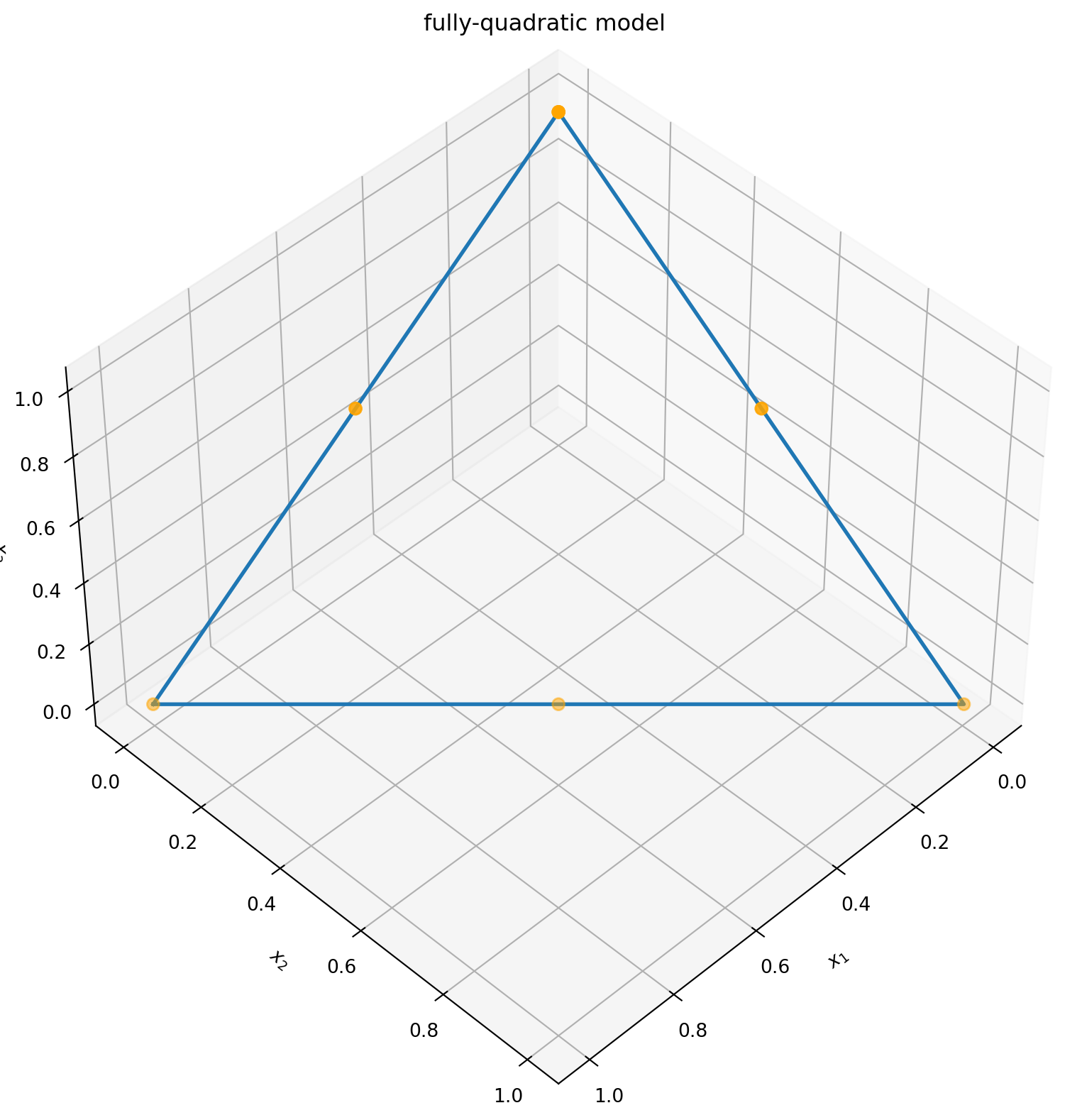
As a simple example for the DoE functionalities we consider the task of finding a D-optimal design for a fully-quadratic model with three design variables with bounds (0,1) and a mixture constraint.
We define the design space including the constraint as a domain. Then we pass it to the optimization routine and specify the model. If the user does not indicate a number of experiments it will be chosen automatically based on the number of model terms.
import numpy as np

from bofire.data_models.strategies.api import DoEStrategy
from bofire.data_models.strategies.doe import DOptimalityCriterion


domain = Domain.from_lists(inputs=[x1, x2, x3], outputs=[y1], constraints=[constr1])
data_model = DoEStrategy(
    domain=domain,
    criterion=DOptimalityCriterion(formula="fully-quadratic"),
)
strategy = strategies.map(data_model=data_model)
candidates = strategy.ask(candidate_count=12)
np.round(candidates, 3)| conc_A | conc_B | conc_C | |
|---|---|---|---|
| 0 | 0.5 | 0.5 | 0.0 |
| 1 | 1.0 | 0.0 | 0.0 |
| 2 | 1.0 | 0.0 | 0.0 |
| 3 | 0.0 | 1.0 | 0.0 |
| 4 | 1.0 | 0.0 | 0.0 |
| 5 | 0.5 | 0.5 | 0.0 |
| 6 | 0.5 | 0.0 | 0.5 |
| 7 | 1.0 | 0.0 | 0.0 |
| 8 | 1.0 | 0.0 | 0.0 |
| 9 | 0.0 | 0.0 | 1.0 |
| 10 | 0.0 | 0.0 | 1.0 |
| 11 | 0.0 | 0.5 | 0.5 |
The resulting design looks like this:
import matplotlib.pyplot as plt


fig = plt.figure(figsize=((10, 10)))
ax = fig.add_subplot(111, projection="3d")
ax.view_init(45, 45)
ax.set_title("fully-quadratic model")
ax.set_xlabel("$x_1$")
ax.set_ylabel("$x_2$")
ax.set_zlabel("$x_3$")
plt.rcParams["figure.figsize"] = (10, 8)

# plot feasible polytope
ax.plot(xs=[1, 0, 0, 1], ys=[0, 1, 0, 0], zs=[0, 0, 1, 0], linewidth=2)

# plot D-optimal solutions
ax.scatter(
    xs=candidates[x1.key],
    ys=candidates[x2.key],
    zs=candidates[x3.key],
    marker="o",
    s=40,
    color="orange",
)