---
title: Multi-fidelity Bayesian Optimization
jupyter: python3
---
```{python}
#| papermill: {duration: 2.980124, end_time: '2024-10-10T20:34:18.797038', exception: false, start_time: '2024-10-10T20:34:15.816914', status: completed}
#| tags: []
import os

import numpy as np
import pandas as pd
from tqdm import tqdm

import bofire.strategies.api as strategies
from bofire.benchmarks.api import Ackley, Benchmark, Branin
from bofire.data_models.acquisition_functions.api import qLogEI
from bofire.data_models.domain.api import Domain
from bofire.data_models.features.api import CategoricalTaskInput
from bofire.data_models.surrogates.api import BotorchSurrogates, MultiTaskGPSurrogate
```
```{python}
#| papermill: {duration: 0.262804, end_time: '2024-10-10T20:34:19.062415', exception: false, start_time: '2024-10-10T20:34:18.799611', status: completed}
#| tags: []
import matplotlib.pyplot as plt
from matplotlib.axes import Axes
```
```{python}
SMOKE_TEST = os.environ.get("SMOKE_TEST")
NUM_INIT_HF = 4
NUM_INIT_LF = 10
if SMOKE_TEST:
    num_runs = 5
    num_iters = 2
    verbose = False
else:
    num_runs = 10
    num_iters = 10
    verbose = True
```
*This notebook is a sequel to "Transfer Learning in BO".*
# Multi-fidelity Bayesian Optimization
In the previous notebook, we saw how using low-fidelity approximations to our
target function can improve the predictions from our surrogate model, leading to
a faster optimization procedure. In this notebook, we show how we can gain even
further performance gains by querying the cheap low-fidelity approximations during
the BO loop.
## Problem definition
We use the same problem as the transfer learning notebook; optimizing the Branin
benchmark, with a low-fidelity function biased by the Ackley function (with fewer initial
points, to demonstrate the strength of being able to query low fidelities). Below, we
define the problem domain, and the strategies we will use to optimize.
As a baseline, we use the `SoboStrategy` with the `MultiTaskSurrogate`, as in the
previous notebook. We also introduce the `MultiFidelityVarianceBasedStrategy` here, which uses
the same surrogate, but is able to query the lower fidelity functions using a
variance-based acquisition function [Kandasamy et al. 2016, Folch et al. 2023].
Both strategies first select a design point $x$ by optimizing the target fidelity.
The `MultiFidelityVarianceBasedStrategy` then selects the fidelity, $m$, by selecting the
lowest fidelity that has a variance over a fixed threshold. This means that the
strategy will explore the cheapest fidelities first, and only query the expensive
fidelities when there is no information to be gained by the cheap approximations.
```{python}
class BraninMultiTask(Benchmark):
    def __init__(self, low_fidelity_allowed=False, **kwargs):
        super().__init__(**kwargs)
        self._branin = Branin()
        self._ackley = Ackley()
        task_input = CategoricalTaskInput(
            key="task",
            categories=["task_hf", "task_lf"],
            allowed=[True, low_fidelity_allowed],
            fidelities=[0, 1],
        )
        self._domain = Domain(
            inputs=self._branin.domain.inputs + (task_input,),
            outputs=self._branin.domain.outputs,
        )

    def _f(self, candidates: pd.DataFrame) -> pd.DataFrame:
        candidates_no_task = candidates.drop(columns=["task"])
        f_branin = self._branin.f(candidates_no_task)
        f_ackley = self._ackley.f(candidates_no_task)
        bias_scale = np.where(candidates["task"] == "task_hf", 0.0, 0.15).reshape(-1, 1)
        bias_scale = pd.DataFrame(bias_scale, columns=self._domain.outputs.get_keys())
        bias_scale["valid_y"] = 0.0
        return f_branin + bias_scale * f_ackley

    def get_optima(self) -> pd.DataFrame:
        optima = self._branin.get_optima()
        optima["task"] = "task_hf"
        return optima


mf_benchmark = BraninMultiTask(low_fidelity_allowed=True)
tl_benchmark = BraninMultiTask(low_fidelity_allowed=False)
```
```{python}
def create_data_set(seed: int):
    # use the tl_benchmark to sample without the low fidelity
    experiments = tl_benchmark.domain.inputs.sample(
        NUM_INIT_HF + NUM_INIT_LF, seed=seed
    )
    experiments["task"] = np.where(
        experiments.index < NUM_INIT_LF, "task_lf", "task_hf"
    )

    # then use the ml_benchmark to evaluate the low fidelity
    return mf_benchmark.f(experiments, return_complete=True)


create_data_set(0)
```
```{python}
from bofire.data_models.strategies.api import MultiFidelityVarianceBasedStrategy


# It isn't necessary to define the surrogate specs here, as the MFStrategy
# will use a MultiTaskGP by default.

mf_data_model = MultiFidelityVarianceBasedStrategy(
    domain=mf_benchmark.domain,
    acquisition_function=qLogEI(),
    fidelity_thresholds=0.1,
)
mf_data_model.surrogate_specs.surrogates[0].inputs
```
```{python}
from bofire.data_models.strategies.api import SoboStrategy


surrogate_specs = BotorchSurrogates(
    surrogates=[
        MultiTaskGPSurrogate(
            inputs=tl_benchmark.domain.inputs,
            outputs=tl_benchmark.domain.outputs,
        )
    ]
)

tl_data_model = SoboStrategy(
    domain=tl_benchmark.domain,
    acquisition_function=qLogEI(),
    surrogate_specs=surrogate_specs,
)
```
# Multi-fidelity Bayesian Optimisation
We first optimize only on the target fidelity (the "Transfer Learning" baseline).
This uses the `SoboStrategy` defined above.
```{python}
#| papermill: {duration: null, end_time: null, exception: null, start_time: null, status: pending}
#| tags: []
tl_results = pd.DataFrame(columns=pd.MultiIndex.from_tuples([], names=("col", "run")))
for run in range(num_runs):
    seed = 2048 * run + 123
    experiments = create_data_set(seed)

    tl_strategy = strategies.map(tl_data_model)
    tl_strategy.tell(experiments)

    assert tl_strategy.experiments is not None

    pbar = tqdm(range(num_iters), desc="Optimizing")
    for _ in pbar:
        candidate = tl_strategy.ask(1)
        y = tl_benchmark.f(candidate, return_complete=True)
        tl_strategy.tell(y)

        hf_experiments = tl_strategy.experiments[
            tl_strategy.experiments["task"] == "task_hf"
        ]
        regret = hf_experiments["y"].min() - tl_benchmark.get_optima()["y"][0].item()

        pbar.set_postfix({"Regret": f"{regret:.4f}"})

    tl_results["fidelity", f"{run}"] = tl_strategy.experiments["task"]
    tl_results["y", f"{run}"] = tl_strategy.experiments["y"]
```
We now repeat the experiment using multi-fidelity BO, allowing the strategy to query
the low fidelity function as well as the high fidelity function:
```{python}
#| papermill: {duration: null, end_time: null, exception: null, start_time: null, status: pending}
#| tags: []
mf_results = pd.DataFrame(columns=pd.MultiIndex.from_tuples([], names=("col", "run")))
for run in range(num_runs):
    seed = 2048 * run + 123
    experiments = create_data_set(seed)

    mf_strategy = strategies.map(mf_data_model)
    mf_strategy.tell(experiments)

    assert mf_strategy.experiments is not None

    pbar = tqdm(range(num_iters), desc="Optimizing")
    for _ in pbar:
        candidate = mf_strategy.ask(1)
        y = mf_benchmark.f(candidate, return_complete=True)
        mf_strategy.tell(y)

        hf_experiments = mf_strategy.experiments[
            mf_strategy.experiments["task"] == "task_hf"
        ]
        regret = hf_experiments["y"].min() - mf_benchmark.get_optima()["y"][0].item()

        pbar.set_postfix({"Regret": f"{regret:.4f}"})

    mf_results["fidelity", f"{run}"] = mf_strategy.experiments["task"]
    mf_results["y", f"{run}"] = mf_strategy.experiments["y"]
```
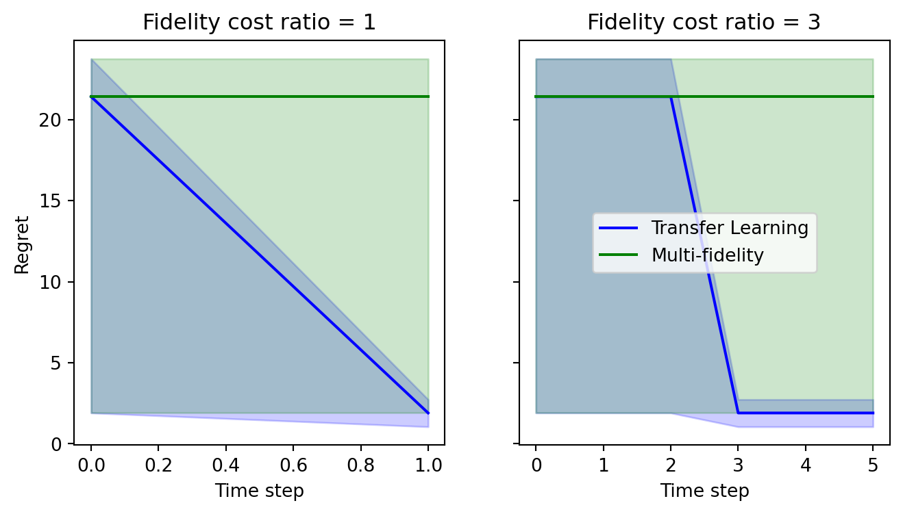
When evaluating the performance, we need to consider how cheap the low-fidelity (LF) is
to query. When the LF has the same cost as the target fidelity, then we
gain very little from the multi-fidelity approach. However, if the LF is cheaper
than the target (in the example below, 3x cheaper) then we observe an improvement in
BO performance.
Specifically, although both strategies have a budget of 10 function queries, the MF
approach uses some of them on
```{python}
#| papermill: {duration: null, end_time: null, exception: null, start_time: null, status: pending}
#| tags: []
def plot_regret(
    ax: Axes, bo_results: pd.DataFrame, fidelity_cost_ratio: float, **plot_kwargs
):
    cummin = (
        bo_results["y"]
        .where(bo_results["fidelity"] == "task_hf", other=np.inf)
        .cummin(axis=0)
    )
    # only select iterations, and the final training point
    cummin = cummin.iloc[-num_iters - 1 :]
    regret: np.ndarray = (cummin - mf_benchmark.get_optima()["y"][0].item()).to_numpy()

    # keep track of "real time", where low fidelities are cheaper to evaluate.
    time_taken = np.where(bo_results["fidelity"] == "task_hf", fidelity_cost_ratio, 1)[
        -num_iters - 1 :
    ].cumsum(axis=0)
    time_taken -= time_taken[0, 0]  # start from T=0 after training data
    iterations = np.arange(num_iters * fidelity_cost_ratio)
    before_time = time_taken[:, :, np.newaxis] <= iterations[np.newaxis, np.newaxis, :]
    regret_before_time = regret[:, :, np.newaxis] * np.where(before_time, 1.0, np.inf)
    # regret_before_time.shape == (num_iters+1, num_runs, len(iterations))
    # project into time dimension
    regret = regret_before_time.min(axis=0)

    ax.plot(
        iterations,
        np.median(regret, axis=0),
        label=plot_kwargs.get("label"),
        color=plot_kwargs.get("color"),
    )
    ax.fill_between(
        iterations,
        np.quantile(regret, 0.75, axis=0),
        np.quantile(regret, 0.25, axis=0),
        color=plot_kwargs.get("color"),
        alpha=0.2,
    )


fig, axs = plt.subplots(ncols=2, figsize=(8, 4), sharey=True)
cost_ratios = (1, 3)

for ax, cost_ratio in zip(axs, cost_ratios):
    plot_regret(
        ax,
        tl_results,
        fidelity_cost_ratio=cost_ratio,
        label="Transfer Learning",
        color="blue",
    )
    plot_regret(
        ax,
        mf_results,
        fidelity_cost_ratio=cost_ratio,
        label="Multi-fidelity",
        color="green",
    )
    ax.set_xlabel("Time step")
    ax.set_title(f"Fidelity cost ratio = {cost_ratio}")


axs[1].legend()
axs[0].set_ylabel("Regret")

plt.show()
```
We can see that allowing the lower fidelities to be queries leads to stronger optimization performance.
We can also see below that the MF approach only samples the target fidelity in later
iterations, once the variance of the LF has been sufficiently reduced.
```{python}
(mf_results["fidelity"] == "task_hf")[-num_iters:].mean(axis=1) # type: ignore
```