import os

import numpy as np
import pandas as pd
from tqdm import tqdm

import bofire.strategies.api as strategies
import bofire.surrogates.api as surrogates
from bofire.benchmarks.api import Ackley, Branin
from bofire.data_models.acquisition_functions.api import qLogEI
from bofire.data_models.domain.api import Domain, Inputs, Outputs
from bofire.data_models.features.api import ContinuousInput, ContinuousOutput, TaskInput
from bofire.data_models.objectives.api import MaximizeObjective
from bofire.data_models.strategies.api import SoboStrategy
from bofire.data_models.surrogates.api import (
    BotorchSurrogates,
    MultiTaskGPSurrogate,
    SingleTaskGPSurrogate,
)

import matplotlib.pyplot as plt

In this notebook we show how to use BoFire for the purposes of transfer learning Bayesian optimization. In particular, we assume we have a task \(f_2\) with data that is relevant to the optimization of our current task \(f_1\). The procedure is simple, we fit a MultiTask GP to both data-sets, however only carry out the BO on \(f_1\), i.e., we optimize the acquisition functions on on the task \(f_1\).

We build a small data-set using the target task:

\[ f_1(x) = \sin(2 \pi x) \]

And we will have data the second related task:

\[ f_2 = 0.9 \sin(2 \pi x) + 0.2 \cos(3 \pi x) - 0.2 \]

We begin by defining the functions, generating some data, and plotting it. We generate 15 data-points for Task 2 and just 4 data-points for Task 1, all the data-points in Task 1 will be in a restricted area of the space.

def task_1_f(x):
    return np.sin(x * 2 * np.pi)


def task_2_f(x):
    return 0.9 * np.sin(x * 2 * np.pi) - 0.2 + 0.2 * np.cos(x * 3 * np.pi)


x = np.linspace(0, 1, 101)

# generate lots of low fidelity data and a few high fidelity data

task_1_x = np.linspace(0.6, 1, 4)
task_1_y = task_1_f(task_1_x)

task_2_x = np.linspace(0, 1, 15)
task_2_y = task_2_f(task_2_x)

# set the data in the pandas format
experiments = pd.DataFrame(
    {
        "x": np.concatenate([task_1_x, task_2_x]),
        "y": np.concatenate([task_1_y, task_2_y]),
        "task": ["task_1"] * len(task_1_x) + ["task_2"] * len(task_2_x),
    },
)

plt.figure(figsize=(6, 4))

plt.scatter(task_1_x, task_1_y, label="Task 1 data", color="red")
plt.scatter(task_2_x, task_2_y, label="Task 2 data", color="blue")

plt.plot(x, task_1_f(x), label="Task 1", color="red")
plt.plot(x, task_2_f(x), label="Task 2", color="blue")

plt.xlabel("x")
plt.ylabel("y")

plt.legend()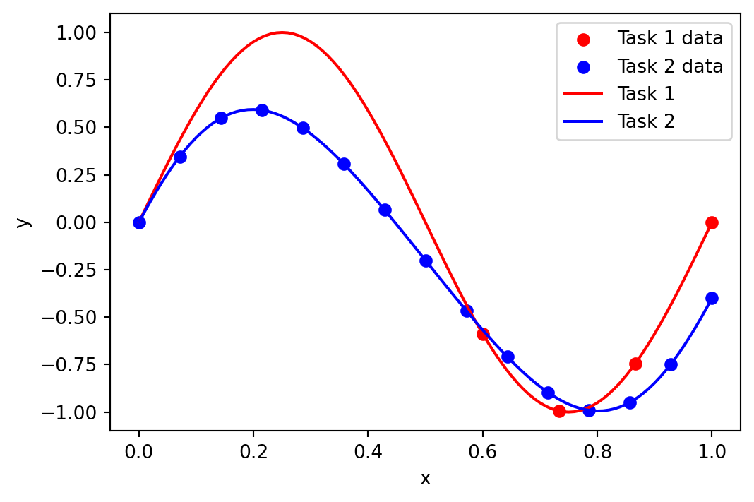

Inference

At first we will show to do inference with the model and see make predictions using multiple data-sets.

We first set-up the model according to BoFire’s API, by defining the set of input and output features and the corresponding bounds, and create a surrogate data model:

• To define the task we choose the TaskInput feature, everything else follows standard BoFire procedure.

# set-up the task model with allowed variable as ["True"] for the target task and ["False"] for the other task
task_input = TaskInput(key="task", categories=["task_1", "task_2"])
# define the input features
input_features = [ContinuousInput(key="x", bounds=(0, 1)), task_input]

objective = MaximizeObjective(w=1)
output_features = [ContinuousOutput(key="y", objective=objective)]

inputs = Inputs(features=input_features)
outputs = Outputs(features=output_features)

surrogate_data = MultiTaskGPSurrogate(inputs=inputs, outputs=outputs)

We map from the surrogate data into the surrogate model and fit the data.

surrogate = surrogates.map(surrogate_data)

surrogate.fit(experiments)

/opt/hostedtoolcache/Python/3.12.12/x64/lib/python3.12/site-packages/linear_operator/utils/interpolation.py:71: UserWarning:

torch.sparse.SparseTensor(indices, values, shape, *, device=) is deprecated.  Please use torch.sparse_coo_tensor(indices, values, shape, dtype=, device=). (Triggered internally at /pytorch/torch/csrc/utils/tensor_new.cpp:654.)

Plot to see how we are able to predict outside of the region where there is data for Task 1, since we can use the data from Task 2 and the learnt correlations:

# predict the high fidelity data
x_predict = np.linspace(0, 1, 101)
y_predict = surrogate.predict(
    pd.DataFrame({"x": x_predict, "task": ["task_1"] * len(x_predict)}),
)

# plot data and predictions
plt.plot(x_predict, y_predict["y_pred"], label="Predictions", color="green")
plt.fill_between(
    x_predict,
    y_predict["y_pred"] - 2 * y_predict["y_sd"],
    y_predict["y_pred"] + 2 * y_predict["y_sd"],
    color="green",
    alpha=0.2,
)

# plot the high fidelity function
plt.plot(x, task_1_f(x), label="Task 1", color="red")

# plot the data too
plt.scatter(
    experiments[experiments["task"] == "task_1"]["x"],
    experiments[experiments["task"] == "task_1"]["y"],
    label="Task 1 data",
    color="red",
)
plt.scatter(
    experiments[experiments["task"] == "task_2"]["x"],
    experiments[experiments["task"] == "task_2"]["y"],
    label="Task 2 data",
    color="blue",
)

plt.xlabel("x")
plt.ylabel("y")

plt.legend()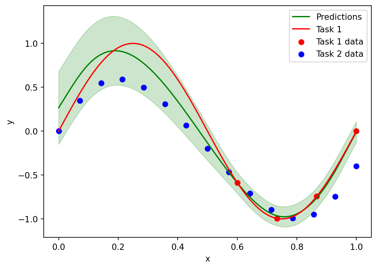

Transfer Learning Bayesian Optimisation

Let us now integrate this into BoFire’s SOBO strategy. This can be done by following the standard BoFire syntax with a small modification.

• For TaskInput we must set the variable allowed as a list, with each element in the list corresponding to one of the categories such that all auxiliary tasks have False and target task has True. For example, we have categories = ["task_1, task_2"] and the goal of our optimization is to optimize task_1 therefore we set allowed = [True, False]:

input_features = [
    ContinuousInput(key="x", bounds=(0, 1)),
    TaskInput(key="task", categories=["task_1", "task_2"], allowed=[True, False]),
]

objective = MaximizeObjective(w=1)
output_features = [ContinuousOutput(key="y", objective=objective)]

inputs = Inputs(features=input_features)
outputs = Outputs(features=output_features)

surrogate_data = MultiTaskGPSurrogate(inputs=inputs, outputs=outputs)
surrogate_specs = BotorchSurrogates(surrogates=[surrogate_data])

# define the acquisition function
acquisition = qLogEI()

sobo_strategy_data_model = SoboStrategy(
    domain=Domain(
        inputs=inputs,
        outputs=outputs,
    ),
    acquisition_function=acquisition,
    surrogate_specs=surrogate_specs,
)

sobo_strategy = strategies.map(sobo_strategy_data_model)

sobo_strategy.tell(experiments)

We can now generate experimental candidates:

candidates = sobo_strategy.ask(3)

candidates

/opt/hostedtoolcache/Python/3.12.12/x64/lib/python3.12/site-packages/botorch/optim/optimize.py:789: RuntimeWarning:

Optimization failed in `gen_candidates_scipy` with the following warning(s):
[NumericalWarning('A not p.d., added jitter of 1.0e-08 to the diagonal'), OptimizationWarning('Optimization failed within `scipy.optimize.minimize` with status 2 and message ABNORMAL: .')]
Trying again with a new set of initial conditions.

	x	task	y_pred	y_sd	y_des
0	0.167697	task_1	0.907478	0.198482	0.907478
1	0.214386	task_1	0.905726	0.192966	0.905726
2	0.189075	task_1	0.916268	0.196207	0.916268

If we instead wanted to optimize task_2 instead of task_1, we simply change allowed = [False, True]:

input_features = [
    ContinuousInput(key="x", bounds=(0, 1)),
    TaskInput(key="task", categories=["task_1", "task_2"], allowed=[False, True]),
]

objective = MaximizeObjective(w=1)
output_features = [ContinuousOutput(key="y", objective=objective)]

inputs = Inputs(features=input_features)
outputs = Outputs(features=output_features)

surrogate_data = MultiTaskGPSurrogate(inputs=inputs, outputs=outputs)
surrogate_specs = BotorchSurrogates(surrogates=[surrogate_data])

# define the acquisition function
acquisition = qLogEI()

sobo_strategy_data_model = SoboStrategy(
    domain=Domain(
        inputs=inputs,
        outputs=outputs,
    ),
    acquisition_function=acquisition,
    surrogate_specs=surrogate_specs,
)

sobo_strategy = strategies.map(sobo_strategy_data_model)

sobo_strategy.tell(experiments)

We now obtain candidates for task_2:

candidate = sobo_strategy.ask(1)

candidate

	x	task	y_pred	y_sd	y_des
0	0.197146	task_2	0.594692	0.026345	0.594692

Let us now run a Bayesian optimization loop on the Branin benchmark to show the usefulness of transfer learning Bayesian optimization in a practical setting. We create a small data-set composed of the Branin benchmark itself, and a large one composed of the Branin function with a small amount of bias added by summing the Branin and Ackley functions.

We begin by defining a function that creates random initial data-sets, and create as many data-sets as the number of runs we want to average over:

benchmark = Branin()
bias = Ackley()


def create_data_set():
    # choose the initial data-sets
    low_fidelity_x = benchmark.domain.inputs.sample(25)
    high_fidelity_x = benchmark.domain.inputs.sample(4)

    # create the observations
    high_fidelity_data = benchmark.f(high_fidelity_x, return_complete=True)
    low_fidelity_bias = bias.f(low_fidelity_x, return_complete=True)

    low_fidelity_data = benchmark.f(low_fidelity_x, return_complete=True)
    low_fidelity_data["y"] = low_fidelity_data["y"] + 0.15 * low_fidelity_bias["y"]

    # create a joint data-set, with the task variable
    high_fidelity_data["task"] = "task_1"
    low_fidelity_data["task"] = "task_2"

    experiments_joint = pd.concat([low_fidelity_data, high_fidelity_data])

    return high_fidelity_data, experiments_joint

single_task_all_regrets = []

SMOKE_TEST = os.environ.get("SMOKE_TEST")
if SMOKE_TEST:
    num_runs = 5
    num_iters = 2
    verbose = False
else:
    num_runs = 10
    num_iters = 10
    verbose = True

# create the initial data-sets for each run

high_fidelity_datasets = []
experiments_joint_datasets = []

for _ in range(num_runs):
    high_fidelity_data, experiments_joint = create_data_set()
    high_fidelity_datasets.append(high_fidelity_data)
    experiments_joint_datasets.append(experiments_joint)

Let us now run a Bayesian optimization loop only using the high-fidelity data:

for run in range(num_runs):
    high_fidelity_data = high_fidelity_datasets[run]

    inputs = benchmark.domain.inputs
    outputs = benchmark.domain.outputs

    surrogate_data = SingleTaskGPSurrogate(inputs=inputs, outputs=outputs)
    surrogate_specs = BotorchSurrogates(surrogates=[surrogate_data])

    acquisition = qLogEI()

    sobo_strategy_data_model = SoboStrategy(
        domain=Domain(
            inputs=inputs,
            outputs=outputs,
        ),
        acquisition_function=acquisition,
        surrogate_specs=surrogate_specs,
    )

    sobo_strategy = strategies.map(sobo_strategy_data_model)

    dataset = high_fidelity_data.drop(columns=["task"])

    sobo_strategy.tell(dataset)

    regrets_single_task = []

    init_regret = (
        sobo_strategy.experiments["y"][sobo_strategy.experiments["y"].argmin()]
        - benchmark.get_optima()["y"][0].item()
    )
    regrets_single_task.append(init_regret)

    pbar = tqdm(range(num_iters), desc="Optimizing")
    for _iter in pbar:
        candidate = sobo_strategy.ask(1)
        y = benchmark.f(candidate, return_complete=True)
        sobo_strategy.tell(y)

        regret = (
            sobo_strategy.experiments["y"][sobo_strategy.experiments["y"].argmin()]
            - benchmark.get_optima()["y"][0].item()
        )
        regrets_single_task.append(regret)

        pbar.set_postfix({"Regret": f"{regret:.4f}"})

    single_task_all_regrets.append(regrets_single_task)

Optimizing:   0%|          | 0/2 [00:00<?, ?it/s]Optimizing:   0%|          | 0/2 [00:00<?, ?it/s, Regret=1.6006]Optimizing:  50%|█████     | 1/2 [00:00<00:00,  2.92it/s, Regret=1.6006]Optimizing:  50%|█████     | 1/2 [00:00<00:00,  2.92it/s, Regret=1.6006]Optimizing: 100%|██████████| 2/2 [00:00<00:00,  2.14it/s, Regret=1.6006]Optimizing: 100%|██████████| 2/2 [00:00<00:00,  2.23it/s, Regret=1.6006]
Optimizing:   0%|          | 0/2 [00:00<?, ?it/s]Optimizing:   0%|          | 0/2 [00:00<?, ?it/s, Regret=8.6227]Optimizing:  50%|█████     | 1/2 [00:00<00:00,  2.86it/s, Regret=8.6227]Optimizing:  50%|█████     | 1/2 [00:01<00:00,  2.86it/s, Regret=8.6227]Optimizing: 100%|██████████| 2/2 [00:01<00:00,  1.89it/s, Regret=8.6227]Optimizing: 100%|██████████| 2/2 [00:01<00:00,  1.99it/s, Regret=8.6227]
Optimizing:   0%|          | 0/2 [00:00<?, ?it/s]Optimizing:   0%|          | 0/2 [00:00<?, ?it/s, Regret=10.5121]Optimizing:  50%|█████     | 1/2 [00:00<00:00,  2.83it/s, Regret=10.5121]Optimizing:  50%|█████     | 1/2 [00:00<00:00,  2.83it/s, Regret=10.5121]Optimizing: 100%|██████████| 2/2 [00:00<00:00,  2.50it/s, Regret=10.5121]Optimizing: 100%|██████████| 2/2 [00:00<00:00,  2.54it/s, Regret=10.5121]
Optimizing:   0%|          | 0/2 [00:00<?, ?it/s]Optimizing:   0%|          | 0/2 [00:00<?, ?it/s, Regret=11.6892]Optimizing:  50%|█████     | 1/2 [00:00<00:00,  2.53it/s, Regret=11.6892]Optimizing:  50%|█████     | 1/2 [00:00<00:00,  2.53it/s, Regret=2.2431] Optimizing: 100%|██████████| 2/2 [00:00<00:00,  2.50it/s, Regret=2.2431]Optimizing: 100%|██████████| 2/2 [00:00<00:00,  2.50it/s, Regret=2.2431]
Optimizing:   0%|          | 0/2 [00:00<?, ?it/s]Optimizing:   0%|          | 0/2 [00:00<?, ?it/s, Regret=4.3216]Optimizing:  50%|█████     | 1/2 [00:00<00:00,  2.80it/s, Regret=4.3216]Optimizing:  50%|█████     | 1/2 [00:00<00:00,  2.80it/s, Regret=1.9281]Optimizing: 100%|██████████| 2/2 [00:00<00:00,  2.74it/s, Regret=1.9281]Optimizing: 100%|██████████| 2/2 [00:00<00:00,  2.74it/s, Regret=1.9281]

We now repeat the experiment but using transfer learning BO:

multitask_all_regrets = []

for run in range(num_runs):
    experiments_joint = experiments_joint_datasets[run]

    input_features = benchmark.domain.inputs.features + [
        TaskInput(key="task", categories=["task_1", "task_2"], allowed=[True, False]),
    ]
    inputs = Inputs(features=input_features)
    outputs = benchmark.domain.outputs

    surrogate_data = MultiTaskGPSurrogate(inputs=inputs, outputs=outputs)
    surrogate_specs = BotorchSurrogates(surrogates=[surrogate_data])

    acquisition = qLogEI()

    sobo_strategy_data_model = SoboStrategy(
        domain=Domain(
            inputs=inputs,
            outputs=outputs,
        ),
        acquisition_function=acquisition,
        surrogate_specs=surrogate_specs,
    )

    sobo_strategy = strategies.map(sobo_strategy_data_model)

    dataset = experiments_joint.copy()

    sobo_strategy.tell(dataset)

    regrets_transfer_learning = []

    # obtain experiments at the highest fidelity
    experiments = sobo_strategy.experiments[
        sobo_strategy.experiments["task"] == "task_1"
    ]["y"]
    init_regret = (
        experiments[experiments.argmin()] - benchmark.get_optima()["y"][0].item()
    )
    regrets_transfer_learning.append(init_regret)

    pbar = tqdm(range(num_iters), desc="Optimizing")
    for _iter in pbar:
        candidate = sobo_strategy.ask(1)
        candidate = candidate.drop(columns=["task"])
        y = benchmark.f(candidate, return_complete=True)
        y["task"] = "task_1"
        sobo_strategy.tell(y)

        experiments = sobo_strategy.experiments[
            sobo_strategy.experiments["task"] == "task_1"
        ]["y"].reset_index(drop=True)
        regret = (
            experiments[experiments.argmin()] - benchmark.get_optima()["y"][0].item()
        )
        regrets_transfer_learning.append(regret)

        pbar.set_postfix({"Regret": f"{regret:.4f}"})

    multitask_all_regrets.append(regrets_transfer_learning)

Optimizing:   0%|          | 0/2 [00:00<?, ?it/s]Optimizing:   0%|          | 0/2 [00:02<?, ?it/s, Regret=1.6006]Optimizing:  50%|█████     | 1/2 [00:02<00:02,  2.28s/it, Regret=1.6006]Optimizing:  50%|█████     | 1/2 [00:04<00:02,  2.28s/it, Regret=1.6006]Optimizing: 100%|██████████| 2/2 [00:04<00:00,  2.01s/it, Regret=1.6006]Optimizing: 100%|██████████| 2/2 [00:04<00:00,  2.05s/it, Regret=1.6006]
Optimizing:   0%|          | 0/2 [00:00<?, ?it/s]Optimizing:   0%|          | 0/2 [00:03<?, ?it/s, Regret=0.0576]Optimizing:  50%|█████     | 1/2 [00:03<00:03,  3.09s/it, Regret=0.0576]Optimizing:  50%|█████     | 1/2 [00:05<00:03,  3.09s/it, Regret=0.0576]Optimizing: 100%|██████████| 2/2 [00:05<00:00,  2.55s/it, Regret=0.0576]Optimizing: 100%|██████████| 2/2 [00:05<00:00,  2.63s/it, Regret=0.0576]
Optimizing:   0%|          | 0/2 [00:00<?, ?it/s]Optimizing:   0%|          | 0/2 [00:01<?, ?it/s, Regret=2.1283]Optimizing:  50%|█████     | 1/2 [00:01<00:01,  1.61s/it, Regret=2.1283]Optimizing:  50%|█████     | 1/2 [00:03<00:01,  1.61s/it, Regret=2.1283]Optimizing: 100%|██████████| 2/2 [00:03<00:00,  1.99s/it, Regret=2.1283]Optimizing: 100%|██████████| 2/2 [00:03<00:00,  1.93s/it, Regret=2.1283]
Optimizing:   0%|          | 0/2 [00:00<?, ?it/s]Optimizing:   0%|          | 0/2 [00:02<?, ?it/s, Regret=4.5466]Optimizing:  50%|█████     | 1/2 [00:02<00:02,  2.77s/it, Regret=4.5466]Optimizing:  50%|█████     | 1/2 [00:05<00:02,  2.77s/it, Regret=1.8311]Optimizing: 100%|██████████| 2/2 [00:05<00:00,  2.52s/it, Regret=1.8311]Optimizing: 100%|██████████| 2/2 [00:05<00:00,  2.56s/it, Regret=1.8311]
Optimizing:   0%|          | 0/2 [00:00<?, ?it/s]Optimizing:   0%|          | 0/2 [00:01<?, ?it/s, Regret=2.9632]Optimizing:  50%|█████     | 1/2 [00:01<00:01,  1.92s/it, Regret=2.9632]Optimizing:  50%|█████     | 1/2 [00:03<00:01,  1.92s/it, Regret=2.9632]Optimizing: 100%|██████████| 2/2 [00:03<00:00,  1.74s/it, Regret=2.9632]Optimizing: 100%|██████████| 2/2 [00:03<00:00,  1.77s/it, Regret=2.9632]

We now plot the quantiles and median simple regret against iteration:

# plot the results
plt.figure(figsize=(6, 4))

regrets_single_task_median = np.median(np.array(single_task_all_regrets), axis=0)
regrets_transfer_learning_median = np.median(np.array(multitask_all_regrets), axis=0)

# get the 25 and 75 percentiles
regrets_single_task_upper_quantile = np.quantile(
    np.array(single_task_all_regrets),
    0.75,
    axis=0,
)
regrets_single_task_lower_quantile = np.quantile(
    np.array(single_task_all_regrets),
    0.25,
    axis=0,
)

regrets_transfer_learning_upper_quantile = np.quantile(
    np.array(multitask_all_regrets),
    0.75,
    axis=0,
)
regrets_transfer_learning_lower_quantile = np.quantile(
    np.array(multitask_all_regrets),
    0.25,
    axis=0,
)

plt.plot(regrets_single_task_median, label="Single task", color="red")
plt.plot(regrets_transfer_learning_median, label="Transfer learning", color="blue")

plt.fill_between(
    np.arange(num_iters + 1),
    regrets_single_task_upper_quantile,
    regrets_single_task_lower_quantile,
    color="red",
    alpha=0.2,
)
plt.fill_between(
    np.arange(num_iters + 1),
    regrets_transfer_learning_upper_quantile,
    regrets_transfer_learning_lower_quantile,
    color="blue",
    alpha=0.2,
)

plt.xlabel("Iteration")
plt.ylabel("Regret")

plt.legend()

plt.show()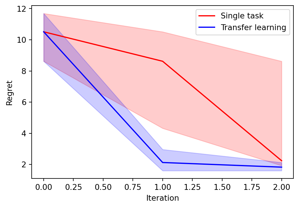

We can see that using transfer learning leads to significant improvement.