import bofire.strategies.api as strategies
from bofire.data_models.api import Domain, Inputs
from bofire.data_models.features.api import ContinuousInput
from bofire.data_models.strategies.api import DoEStrategy
from bofire.data_models.strategies.doe import DOptimalityCriterion
from bofire.utils.doe import get_confounding_matrixDesign with explicit Formula
This tutorial notebook shows how to setup a D-optimal design with BoFire while providing an explicit formula and not just one of the four available keywords linear, linear-and-interaction, linear-and-quadratic, fully-quadratic.
Make sure that cyipoptis installed. The recommend way is the installation via conda conda install -c conda-forge cyipopt.
Imports
Setup of the problem
input_features = Inputs(
    features=[
        ContinuousInput(key="a", bounds=(0, 5)),
        ContinuousInput(key="b", bounds=(40, 800)),
        ContinuousInput(key="c", bounds=(80, 180)),
        ContinuousInput(key="d", bounds=(200, 800)),
    ],
)
domain = Domain(inputs=input_features)
Definition of the formula for which the optimal points should be found
model_type = "a + {a**2} + b + c + d + a:b + a:c + a:d + b:c + b:d + c:d"
model_type
'a + {a**2} + b + c + d + a:b + a:c + a:d + b:c + b:d + c:d'Find D-optimal Design
data_model = DoEStrategy(
    domain=domain,
    criterion=DOptimalityCriterion(formula=model_type),
    ipopt_options={"max_iter": 100, "print_level": 0},
)
strategy = strategies.map(data_model=data_model)
design = strategy.ask(17)
design
/opt/hostedtoolcache/Python/3.12.13/x64/lib/python3.12/site-packages/bofire/strategies/doe/utils.py:819: OptimizeWarning: Unknown solver options: disp
result = opt.minimize(| a | b | c | d | |
|---|---|---|---|---|
| 0 | 5.000000 | 800.000000 | 180.0 | 224.040097 |
| 1 | 0.000000 | 675.603491 | 180.0 | 200.000000 |
| 2 | 0.000000 | 800.000000 | 180.0 | 589.995620 |
| 3 | 0.000000 | 40.000000 | 80.0 | 200.000000 |
| 4 | 5.000000 | 40.000000 | 180.0 | 800.000000 |
| 5 | 0.000000 | 800.000000 | 80.0 | 800.000000 |
| 6 | 0.000000 | 40.000000 | 180.0 | 794.397813 |
| 7 | 5.000000 | 40.000000 | 80.0 | 236.606559 |
| 8 | 5.000000 | 800.000000 | 80.0 | 800.000000 |
| 9 | 2.692361 | 563.976784 | 180.0 | 800.000000 |
| 10 | 5.000000 | 40.000000 | 180.0 | 200.000000 |
| 11 | 2.579562 | 420.147984 | 180.0 | 200.000000 |
| 12 | 5.000000 | 749.559960 | 80.0 | 200.000000 |
| 13 | 0.000000 | 40.000000 | 180.0 | 343.173183 |
| 14 | 0.000000 | 800.000000 | 80.0 | 200.000000 |
| 15 | 2.632074 | 40.000000 | 80.0 | 800.000000 |
| 16 | 5.000000 | 800.000000 | 180.0 | 384.010613 |
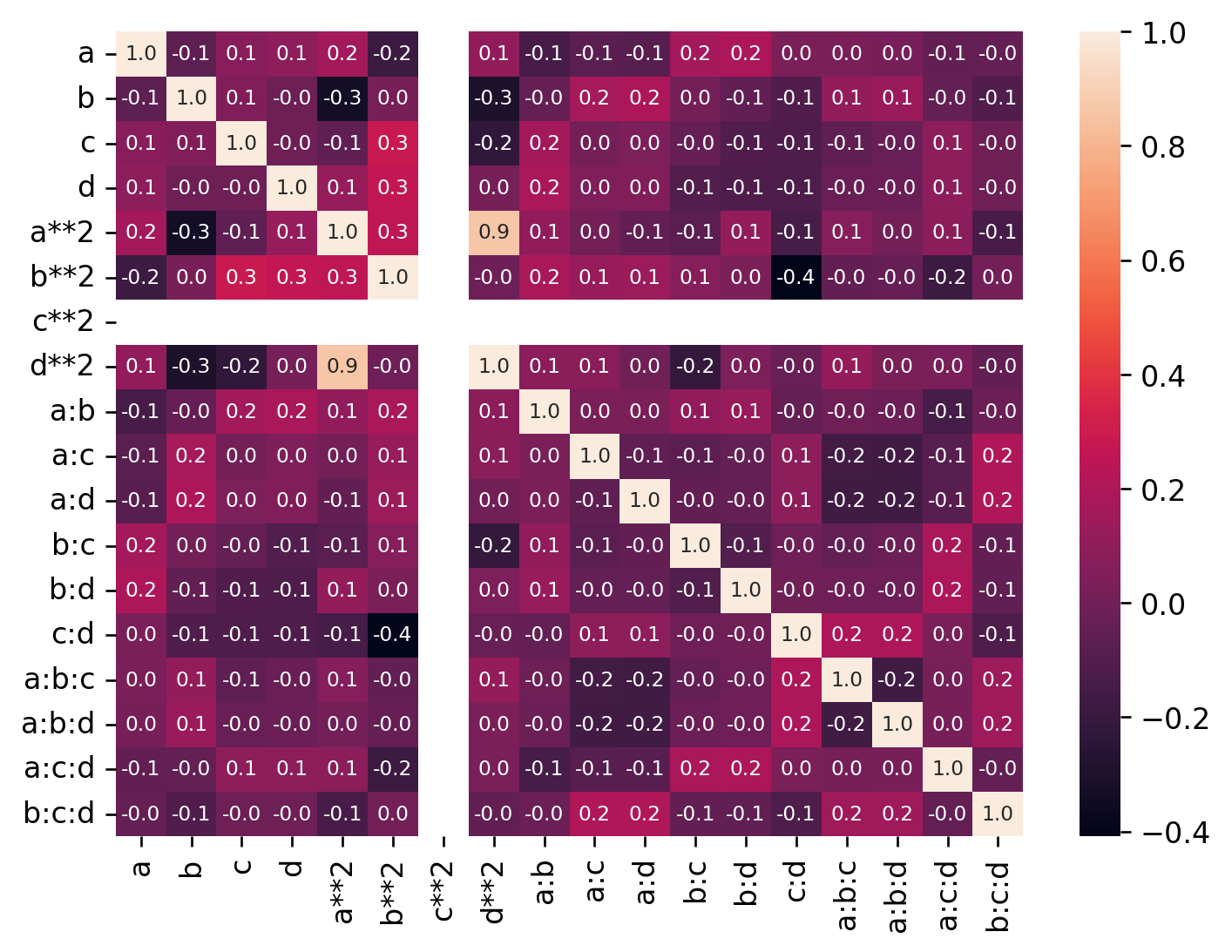
Analyze Confounding
import matplotlib
import matplotlib.pyplot as plt
import seaborn as sns


matplotlib.rcParams["figure.dpi"] = 120

m = get_confounding_matrix(
    domain.inputs,
    design=design,
    interactions=[2, 3],
    powers=[2],
)

sns.heatmap(m, annot=True, annot_kws={"fontsize": 7}, fmt="2.1f")
plt.show()