import numpy as np
import pandas as pd
import shap

import bofire.surrogates.api as surrogates
from bofire.data_models.domain.api import Inputs, Outputs
from bofire.data_models.enum import RegressionMetricsEnum
from bofire.data_models.features.api import ContinuousInput, ContinuousOutput
from bofire.data_models.surrogates.api import SingleTaskGPSurrogate
from bofire.plot.cv_folds import plot_cv_folds_plotly
from bofire.plot.feature_importance import plot_feature_importance_by_feature_plotly
from bofire.plot.gp_slice import plot_gp_slice_plotly
from bofire.surrogates.feature_importance import (
    combine_lengthscale_importances,
    combine_permutation_importances,
    lengthscale_importance_hook,
    permutation_importance_hook,
    shap_importance,
    shap_importance_hook,
)Model Building with BoFire
This notebooks shows how to setup and analyze models trained with BoFire.
Imports
Problem Setup
For didactic purposes, we sample data from a Himmelblau benchmark function and use them to train a SingleTaskGP.
input_features = Inputs(
    features=[ContinuousInput(key=f"x_{i+1}", bounds=(-4, 4)) for i in range(3)],
)
output_features = Outputs(features=[ContinuousOutput(key="y")])
experiments = input_features.sample(n=50)
experiments.eval("y=((x_1**2 + x_2 - 11)**2+(x_1 + x_2**2 -7)**2)", inplace=True, engine = "python")
experiments["valid_y"] = 1

experiments["labcode"] = "exp_" + experiments.index.astype(str)
Cross Validation
Run the cross validation
data_model = SingleTaskGPSurrogate(
    inputs=input_features,
    outputs=output_features,
)

model = surrogates.map(data_model=data_model)
train_cv, test_cv, pi = model.cross_validate(
    experiments,
    folds=5,
    include_X = True,
    include_labcodes = True,
    hooks={
        "permutation_importance": permutation_importance_hook,
        "lengthscale_importance": lengthscale_importance_hook,
        "shap_importance": shap_importance_hook,
    },
)
/opt/hostedtoolcache/Python/3.12.13/x64/lib/python3.12/site-packages/bofire/surrogates/botorch.py:185: UserWarning: The given NumPy array is not writable, and PyTorch does not support non-writable tensors. This means writing to this tensor will result in undefined behavior. You may want to copy the array to protect its data or make it writable before converting it to a tensor. This type of warning will be suppressed for the rest of this program. (Triggered internally at /pytorch/torch/csrc/utils/tensor_numpy.cpp:213.)
torch.from_numpy(Y.values).to(**tkwargs),Plot feature importance
shap_folds = pi["shap_importance"]  # list[dict[str, shap.Explanation]]
shap_mean_abs_per_fold = pd.DataFrame(
    [
        pd.Series(
            np.mean(np.abs(fold["y"].values), axis=0),
            index=fold["y"].feature_names,
        )
        for fold in shap_folds
    ]
)

combined_importances = {
    m.name: combine_permutation_importances(pi["permutation_importance"], m).describe()
    for m in RegressionMetricsEnum
}
combined_importances["lengthscale"] = combine_lengthscale_importances(
    pi["lengthscale_importance"],
).describe()
combined_importances["shap"] = shap_mean_abs_per_fold.describe()

plot_feature_importance_by_feature_plotly(
    combined_importances,
    relative=False,
    caption="Feature Importances",
    show_std=True,
    importance_measure="Importance",
)
Analyze the cross validation
# Performance on test sets
test_cv.get_metrics(combine_folds=False)| MAE | MSD | R2 | MAPE | PEARSON | SPEARMAN | FISHER | |
|---|---|---|---|---|---|---|---|
| 0 | 4.236435 | 44.996337 | 0.987771 | 0.457160 | 0.995214 | 1.000000 | 0.003968 |
| 1 | 5.808744 | 48.224472 | 0.971355 | 0.100042 | 0.985674 | 0.963636 | 0.003968 |
| 2 | 7.603971 | 114.063586 | 0.944055 | 0.084335 | 0.978034 | 0.951515 | 0.003968 |
| 3 | 16.813133 | 1116.188163 | 0.824798 | 0.753149 | 0.943292 | 0.866667 | 0.103175 |
| 4 | 12.205448 | 225.836144 | 0.898378 | 0.174838 | 0.962327 | 0.963636 | 0.103175 |
display(test_cv.get_metrics(combine_folds=False))
display(test_cv.get_metrics(combine_folds=False).describe())| MAE | MSD | R2 | MAPE | PEARSON | SPEARMAN | FISHER | |
|---|---|---|---|---|---|---|---|
| 0 | 4.236435 | 44.996337 | 0.987771 | 0.457160 | 0.995214 | 1.000000 | 0.003968 |
| 1 | 5.808744 | 48.224472 | 0.971355 | 0.100042 | 0.985674 | 0.963636 | 0.003968 |
| 2 | 7.603971 | 114.063586 | 0.944055 | 0.084335 | 0.978034 | 0.951515 | 0.003968 |
| 3 | 16.813133 | 1116.188163 | 0.824798 | 0.753149 | 0.943292 | 0.866667 | 0.103175 |
| 4 | 12.205448 | 225.836144 | 0.898378 | 0.174838 | 0.962327 | 0.963636 | 0.103175 |
| MAE | MSD | R2 | MAPE | PEARSON | SPEARMAN | FISHER | |
|---|---|---|---|---|---|---|---|
| count | 5.000000 | 5.000000 | 5.000000 | 5.000000 | 5.000000 | 5.000000 | 5.000000 |
| mean | 9.333546 | 309.861740 | 0.925271 | 0.313905 | 0.972908 | 0.949091 | 0.043651 |
| std | 5.137807 | 456.663788 | 0.065576 | 0.287766 | 0.020469 | 0.049534 | 0.054338 |
| min | 4.236435 | 44.996337 | 0.824798 | 0.084335 | 0.943292 | 0.866667 | 0.003968 |
| 25% | 5.808744 | 48.224472 | 0.898378 | 0.100042 | 0.962327 | 0.951515 | 0.003968 |
| 50% | 7.603971 | 114.063586 | 0.944055 | 0.174838 | 0.978034 | 0.963636 | 0.003968 |
| 75% | 12.205448 | 225.836144 | 0.971355 | 0.457160 | 0.985674 | 0.963636 | 0.103175 |
| max | 16.813133 | 1116.188163 | 0.987771 | 0.753149 | 0.995214 | 1.000000 | 0.103175 |
Plot Folds
plot_cv_folds_plotly(test_cv, plot_X=True, plot_labcodes=True, plot_uncertainties=True)Plot a slice of the GP
In this slice plot, we vary the inputs x_1 and x_2 across their full bounds to create a grid, while keeping x_3 fixed at a selected value.
The outputs are two Plotly figures: one showing the GP’s predicted mean (fig_mean) and the other showing the predicted standard deviation or uncertainty (fig_sd) over the slice.
If observed_data=experiments is provided, the mean plot will also display the measured data points, with those matching the fixed value of x_3 highlighted separately.
fixed_input_features = [model.inputs.get_by_key("x_3")]
fixed_values = [0.0]
varied_input_features = [
model.inputs.get_by_key("x_1"),
model.inputs.get_by_key("x_2"),
]
output_feature = model.outputs.get_by_key("y")
fixed_values = [experiments.iloc[0]["x_3"]]
fig_mean, fig_sd = plot_gp_slice_plotly(
surrogate=model,
fixed_input_features=fixed_input_features,
fixed_values=fixed_values,
varied_input_features=varied_input_features,
output_feature=output_feature,
resolution=80,
observed_data=experiments,
)
display(fig_mean)
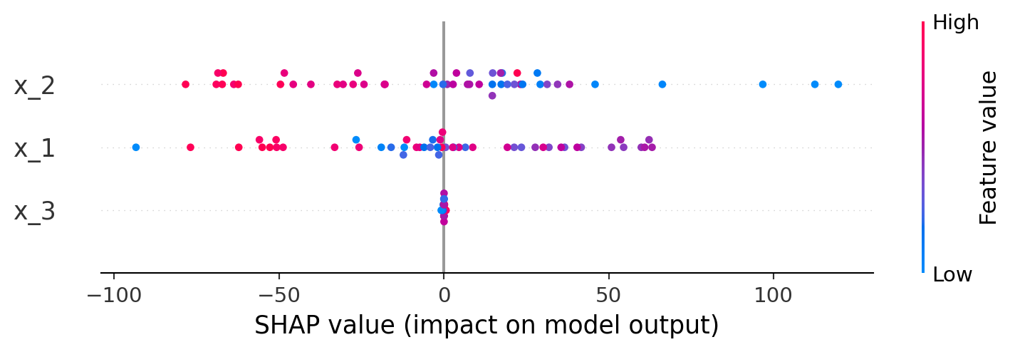
display(fig_sd)Shapley Plots
shap_explanations = shap_importance(
    predictor=model,
    experiments=experiments,
    bg_experiments=experiments,   # background for KernelSHAP
    bg_sample_size=50,
    seed=42,
)

exp = shap_explanations['y']
shap.summary_plot(exp.values, exp.data, feature_names=exp.feature_names)